[이재우] Instacart 그래프 그리기와 해석

# 1. Introduction
[Instacart](https://en.wikipedia.org/wiki/Instacart) 는 미국의 큰 grocery shop 중의 하나이다. 이 회사에서 open dataset 인 "[The Instacart Online Grocery Shopping Dataset 2017](https://tech.instacart.com/3-million-instacart-orders-open-sourced-d40d29ead6f2)" 을 발표하였다. 발표된 내용에는 아래와 같은 내용이 있었다.
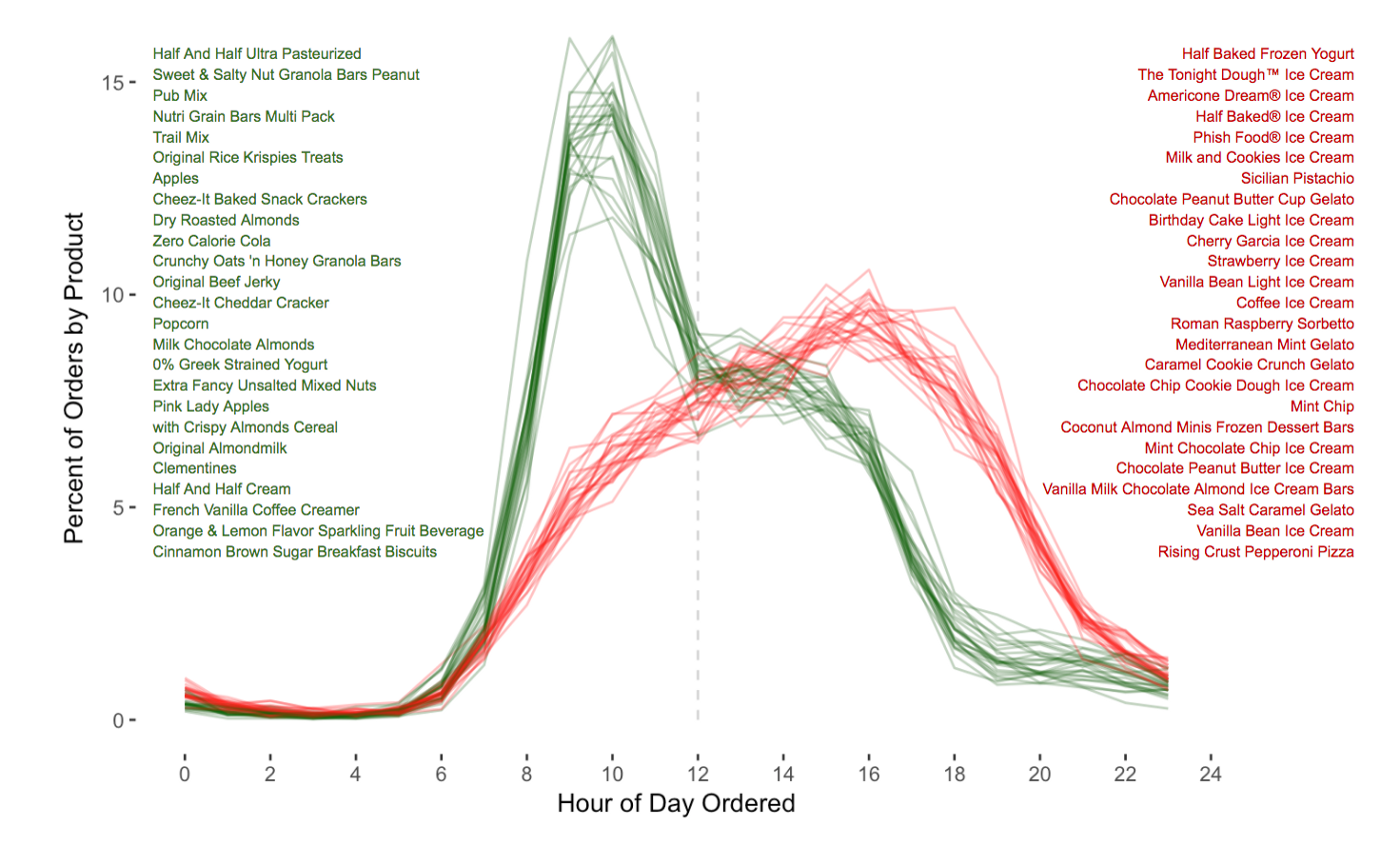
> In fact, of the top 25 latest ordered products, the first 24 are ice cream! The last one, of course, is a frozen pizza.

[Kaggle](https://www.kaggle.com/shwong/the-instacart-chart) 에서 이 그래프를 python 똑같이 구현한 노트북이 있다. 그것을 참고하여, 위의 그래프를 똑같이 그려보고, _In fact, of the top 25 latest ordered products, the first 24 are ice cream! The last one, of course, is a frozen pizza_ 의 의미를 해석해보자.

# 2. graph plotting ( [dataset](https://s3.amazonaws.com/instacart-datasets/instacart_online_grocery_shopping_2017_05_01.tar.gz) , [data dictionary](https://gist.github.com/jeremystan/c3b39d947d9b88b3ccff3147dbcf6c6b) )
## 2.1 import library and data
```py
import os
import pandas as pd
import matplotlib.pyplot as plt

%matplotlib inline

pd.set_option('display.width', 1000)

df_order_products__prior = pd.read_csv('order_products__prior.csv')
df_order_products__train = pd.read_csv('order_products__train.csv')
df_orders = pd.read_csv('orders.csv')
df_products = pd.read_csv('products.csv')
```
## 2.2 Data Organizing
```py
# df_orders.eval_set 의 데이터 값이 'test' 인 행 삭제
df_orders = df_orders[df_orders.eval_set != 'test']

# 열의 이름이 'eval_set' 인 열을 삭제
df_orders = df_orders.drop(['eval_set'], axis=1)

# df_order_products_prior 과 df_order_products_train 합치기
df_order_products = pd.concat([df_order_products__prior, df_order_products__train])

# 'order_id' 를 기준으로 df_orders와 df_order_products 를 합치기
df = df_orders.merge(df_order_products, on='order_id')
print(df.head())
```
> [out put]:

  order_id | user_id | order_number | order_dow | order_hour_of_day | days_since_prior_order | product_id | add_to_cart_order | reordered
| -- | -- | -- | -- | -- | -- | -- | -- | --
2539329 | 1 | 1 | 2 | 8 | NaN | 196 | 1 | 0
2539329 | 1 | 1 | 2 | 8 | NaN | 14084 | 2 | 0
2539329 | 1 | 1 | 2 | 8 | NaN | 12427 | 3 | 0
2539329 | 1 | 1 | 2 | 8 | NaN | 26088 | 4 | 0
2539329 | 1 | 1 | 2 | 8 | NaN | 26405 | 5 | 0

df_orders 에서 고객의 분류가 test 로 된 항목을 다 제거하였다. 이는, df_order_products_prior, df_order_products_train 에서 알 수 있듯이 고객의 분류가 prior 또는 train 의 데이터만 있기 때문이다. 이 그래프를 그리기 위해서는 고객의 분류가 의미가 없어서, 삭제를해주었다. 따라서 df_order_products_prior 과 df_order_products_train 를 하나의 df_order_products 로 합친 것도 이해가 될 수 있다. 그리고 df 를 정의하였는데, 이는 df_orders 에 df_order_products 를 order_id 를 통해서 합친것을 알 수 있다.
여기서 기술적으로 이해되어야 할 부분이 한 가지 있다. `pd.concat` 과 `pd.merge` 이다. 왜 df_order_products 는 `concat` 을 사용하고, df 는 `merge` 를 사용했을까? 먼저 엑셀로 비유해서 설명하면, `concat`은 서로 다른 sheet 있는 정보들을 하나의 sheet 에 Ctrl + c, Ctrl + v 한 것이다. 하지만 `merge`는 엑셀의 vlookup 함수와 같다. vlookup 함수는 특정값을 지정해주고, 그 특정 값을 다른 데이터에서 찾아서 원하는 값을 불러오는 것이다. 이처럼, `merge` 는 df_orders 에서 order_id 를 df_order_products 에서 찾아서 df_orders_products 의 값들을
df_orders 에 붙이는 것이다.
## 2.3 Reducing the problem size
```py
## 판매 횟수가 가장 높은 2000 개의 물품만으로 데이터 자체를 축소 시켰다.
top_products = pd.DataFrame({'total_count': df.groupby('product_id').size()}).sort_values('total_count', ascending=False).reset_index()[:2000]
top_products = top_products.merge(df_products, on='product_id')
print(top_products.head())
```
>[out put]:

 product_id | total_count | product_name | aisle_id | department_id
| -- | -- | -- | -- | --
24852 | 491291 | Banana | 24 | 4
13176 | 394930 | Bag of Organic Bananas | 24 | 4
21137 | 275577 | Organic Strawberries | 24 | 4
21903 | 251705 | Organic Baby Spinach | 123 | 4
47209 | 220877 | Organic Hass Avocado | 24 | 4

여기서는 top_products 라는 새로운 DataFrame 을 정의 하였는데, 이는 df 에서 product_id 를 기준으로 각 각의 total_count 를 보여주는 데이터이다. `groupby` 는 기준 설정을, `size()`는 count를 도와준다. 마지막으로 `sort_values('total_count', ascending=False)`를 통해서 total_count 를 기준으로 내림차순으로 정렬 하였다. 마지막으로 `reset_index()[:2000]` 은 정렬된 데이터로 새로 indexing 을 하여서, 상위 2000개의 data 만 사용하겠다는 것이다. 이렇게 정의된 top_products 는 구매 횟수가 Top 2000 인 물품들의 주문만 담겨져 있는 데이터가 되는 것이다. 게다가 top_products 에 df_products 를 `merge` 하면서, df_products 에 있는 정보도 합쳐주었다. 기술적인 부분에서

* `pd.DataFrame({'total_count': df.groupby('product_id').size()}).sort_values('total_count', ascending=False).reset_index()[:2000]` 은 유용한 방법중의 하나이다.

대부분 count 라고 생각하면 `value_counts()` 를 먼저 생각할 수 있는데, 이 분은 하나의 새로운 데이터 세트를 정의하면서, DataFrame 타입을 유지하는 방법을 자주 사용한다. 이와 똑같은 코드를 `df.product_id.value_counts(ascending=False)` 로 할 수 있지만 이 것의 결과는 DataFrame이 아닌 Series 이므로 차이가 있다.

## 2.3 Product and Hour of Day Distribution
```py
# df에 상위 2000개의 해당하는 product_id 를 가진 주문만 보도록 설정하는것
df = df.loc[df['product_id'].isin(top_products.product_id)]
# df 에서 proudct_id 와 order_hour_of_day 를 기준으로 count를 확인 할 수 있는 데이터 프레임
product_orders_by_hour = pd.DataFrame({'count': df.groupby(['product_id', 'order_hour_of_day']).size()}).reset_index()
product_orders_by_hour['pct'] = product_orders_by_hour.groupby('product_id')['count'].apply(lambda x: x/x.sum()*100)
product_orders_by_hour.head()
```
>[out put] :

product_id | order_hour_of_day | count | pct
| -- | -- | -- | --
34 | 0 | 23 | 0.339283
34 | 1 | 18 | 0.265526
34 | 2 | 11 | 0.162266
34 | 3 | 5 | 0.073757
34 | 4 | 5 | 0.073757

product_orders_by_hour 라는 데이터 프레임은, 이전의 방법과 같이 'product_id' 와 'order_hour_of_day' 를 기준으로 product_id 가 몇번 나왔는지 `size()` 를 통해서 count 한 다음 그 값을 함께 저장한 데이터 세트이다. product_orders_by_hour 에 'pct' 라는 column 을 추가했다. 이는 product_id 별로 각 시간대의 주문의 횟수가 해당 물품의 총 주문의 몇퍼센트 인지 나타내는 열이다. 여기에서는

* `product_orders_by_hour.groupby('product_id')['count'].apply(lambda x: x/x.sum()*100)` 를 사용하였는데,

`lambda` 함수의 목적은 따로 정의 하지않고 1회용의 함수를 사용할 때 많이 사용한다. 여기서 **x** 는 argument 이고 결과로 **x/x.sum()*100** 반환 한다는 뜻이다. **x** 의 값은 product_orders_by_hour['count'] 이 될 것이다. 여기서도 이 분은 새로 데이터 세트로 정의를 하였다. 보여주는 이해를 돕기 위해서인지 알기는 어려우나, 이 과정을 통해 보여지는 결과를 통해서 이해하기 쉬운것은 사실이다.

```py
mean_hour = pd.DataFrame({'mean_hour': product_orders_by_hour.groupby('product_id').apply(lambda x: sum(x['order_hour_of_day'] * x['count'])/sum(x['count']))}).reset_index()
print(mean_hour.head())
```
>[out put]:

  product_id | mean_hour
| -- | --
34 | 13.511285
45 | 13.398624
79 | 13.502530
116 | 12.516822
117 | 13.392173

mean_hour 는 product_id 별로 구매시간의 평균을 나타내는 dataframe 이다. `groupby` 를 통해서 product_id 를 기준으로 잡고, `apply()` 를 통해서 새로운 함수를 적용 시킬 것이며, `lambda x : sum(x['order_hour_of_day'] * x['count'])/sum(x['count']))}` 는 [frequency table](https://www.mathsisfun.com/data/mean-frequency-table.html) 의 평균을 구하는 방법이다. 여기서 x 의 값은 product_orders 인 데이터 프레임이 될 것이다. 기술적인 부분에서는

* `pd.DataFrame({'mean_hour': product_orders_by_hour.groupby('product_id').apply(lambda x: sum(x['order_hour_of_day'] * x['count'])/sum(x['count']))}).reset_index()` 의 활용이다.

여기서는 `groupby` 와 `apply()` 의 또 다른 적용 방법이다. 앞의 과정에서는 `lambda` 에서 받아지는 **x** 의 값이 product_orders_by_hour['count'] 였지만, 이 경우에는 **x** 의 값은 product_orders_by_hour 데이터 세트 전체이다. 그렇기 때문에 `lambda x: sum(x['order_hour_of_day'] * x['count'])/sum(x['count']))` 에서 `x['count'] 또는 x['order_hour_of_day`] 를 쓸 수 있는 이유이다.

```py
morning = mean_hour.sort_values('mean_hour')[:25]
morning = morning.merge(df_products, on='product_id')
morning.head()
```
>[out put]:

  product_id | mean_hour | product_name | aisle_id | department_id
| -- | -- | -- | -- | --
9292 | 11.767279 | Half And Half Ultra Pasteurized | 84 | 16
46562 | 11.898340 | Sweet & Salty Nut Granola Bars Peanut | 3 | 19
45051 | 12.004019 | Pub Mix | 107 | 19
36472 | 12.049459 | Nutri Grain Bars Multi Pack | 48 | 14
37710 | 12.059043 | Trail Mix | 125 | 19

mean_hour 를 기준으로 평균시간이 작은 상위 25개를 뽑은 것을 morning 이라고 저장한다. 그런다음 product_id 를 기준으로 df_products 로 `merge` 해서 product_name 을 확인할 수 있다.

```py
afternoon = mean_hour.sort_values('mean_hour', ascending=False)[:25]
afternoon = afternoon.merge(df_products, on='product_id')
afternoon.head()
```
>[out put]:

| product_id | mean_hour | product_name | aisle_id | department_id
| -- | -- | -- | -- | --
30668 | 14.526986 | Half Baked Frozen Yogurt | 37 | 1
45541 | 14.526299 | The Tonight Dough™ Ice Cream | 37 | 1
45681 | 14.394912 | Americone Dream® Ice Cream | 37 | 1
46175 | 14.388942 | Half Baked® Ice Cream | 37 | 1
14335 | 14.373308 | Phish Food® Ice Cream | 37 | 1

mean_hour 를 기준으로 평균 시간이 큰 상위 25개를 뽑은 것을 afternoon 이라고 저장한다. 그런다음 product_id 를 기준으로 df_products 로 `merge` 해서 product_name 을 확인할 수 있다.

## 2.4 plot
```py
morning_pct = product_orders_by_hour.merge(morning, on='product_id').sort_values(['mean_hour', 'order_hour_of_day'])
afternoon_pct = product_orders_by_hour.merge(afternoon, on='product_id').sort_values(['mean_hour', 'order_hour_of_day'], ascending=False)
```
```py
morning_pct.head()
```
>[out put]:

  product_id | order_hour_of_day | count | pct | mean_hour | product_name | aisle_id | department_id
| -- | -- | -- | -- | -- | -- | -- | --
9292 | 0 | 6 | 0.200334 | 11.767279 | Half And Half Ultra Pasteurized | 84 | 16
9292 | 1 | 1 | 0.033389 | 11.767279 | Half And Half Ultra Pasteurized | 84 | 16
9292 | 2 | 1 | 0.033389 | 11.767279 | Half And Half Ultra Pasteurized | 84 | 16
9292 | 4 | 1 | 0.033389 | 11.767279 | Half And Half Ultra Pasteurized | 84 | 16
9292 | 5 | 4 | 0.133556 | 11.767279 | Half And Half Ultra Pasteurized | 84 | 16

```py
afternoon_pct.head()
```
>[out put]:

  product_id | order_hour_of_day | count | pct | mean_hour | product_name | aisle_id | department_id
| -- | -- | -- | -- | -- | -- | -- | --
30668 | 23 | 36 | 1.206839 | 14.526986 | Half Baked Frozen Yogurt | 37 | 1
30668 | 22 | 49 | 1.642642 | 14.526986 | Half Baked Frozen Yogurt | 37 | 1
30668 | 21 | 86 | 2.883004 | 14.526986 | Half Baked Frozen Yogurt | 37 | 1
30668 | 20 | 147 | 4.927925 | 14.526986 | Half Baked Frozen Yogurt | 37 | 1
30668 | 19 | 198 | 6.637613 | 14.526986 | Half Baked Frozen Yogurt | 37 | 1

plot을 쉽게 하기위해서 morning 과 afternoon 서로 분리 시키기 위한 과정이다. plot을 하기 위해서는 product_orders_by_hour 의 데이터에 각 시간의 데이터 프레임을 product_id 를 기준으로 `merge` 시키고, `sort_values(['mean_hour', 'order_hour_of_day'])` 를 통해서 mean_hour 와 order_hour_of_day 작은 순으로 정렬 되어 있다.

```py
# morning 과 afternoon 에 있는 product_name 을 리스트로 만들어서, \n : 줄바꿈 을 사이사이에 넣어 하나의 string 으로 만들었다.
morning_product_names = list(morning_pct['product_name'].unique())
morning_product_names = '\n'.join(morning_product_names)
afternoon_product_names = list(afternoon_pct['product_name'].unique())
afternoon_product_names = '\n'.join(afternoon_product_names)

# 그래프의 이름들과 일치하기 위해서 'Variety Pack` 의 글자는 지웠다.
morning_product_names = morning_product_names.replace('Variety Pack ', '')
```
```py
print(morning_product_names)
```
>[output]:
Half And Half Ultra Pasteurized
Sweet & Salty Nut Granola Bars Peanut
Pub Mix
Nutri Grain Bars Multi Pack
Trail Mix
Original Rice Krispies Treats
Apples
Cheez-It Baked Snack Crackers
Dry Roasted Almonds
Zero Calorie Cola
Crunchy Oats 'n Honey Granola Bars
Original Beef Jerky
Cheez-It Cheddar Cracker
Popcorn
Milk Chocolate Almonds
0% Greek Strained Yogurt
Extra Fancy Unsalted Mixed Nuts
Pink Lady Apples
with Crispy Almonds Cereal
Original Almondmilk
Clementines
Half And Half Cream
French Vanilla Coffee Creamer
Orange & Lemon Flavor Sparkling Fruit Beverage
Cinnamon Brown Sugar Breakfast Biscuits

```py
print(afternoon_product_names)
```
>[out put]:
Half Baked Frozen Yogurt
The Tonight Dough™ Ice Cream
Americone Dream® Ice Cream
Half Baked® Ice Cream
Phish Food® Ice Cream
Milk and Cookies Ice Cream
Sicilian Pistachio
Chocolate Peanut Butter Cup Gelato
Birthday Cake Light Ice Cream
Cherry Garcia Ice Cream
Strawberry Ice Cream
Vanilla Bean Light Ice Cream
Coffee Ice Cream
Roman Raspberry Sorbetto
Mediterranean Mint Gelato
Caramel Cookie Crunch Gelato
Chocolate Chip Cookie Dough Ice Cream
Mint Chip
Coconut Almond Minis Frozen Dessert Bars
Mint Chocolate Chip Ice Cream
Chocolate Peanut Butter Ice Cream
Vanilla Milk Chocolate Almond Ice Cream Bars
Sea Salt Caramel Gelato
Vanilla Bean Ice Cream
Rising Crust Pepperoni Pizza

위의 그래프처럼 product_name 들이 한 줄에 하나씩 나와있는것을 만들기 위해서 product_name 을 `list()` 로 만든다음 `join` 을 통해서 각 각의 elment 들을 `\n` 줄바꿈으로 연결시켜서 하나의 string 으로 만든 것이다. 기술적인 부분으로는, 데이터 세트의 특정 열의 값을 추출해서 `list()` 를 통해서 list 로 형변화가 가능하며, 그리고 그 list 의 element 의 값이 string 일 경우 `join()` 을 통해서 하나의 string 으로 만들 수 있다는 것이다.

```py
# 그래프의 크기 ( fig = figure , ax = axes )
fig, ax = plt.subplots(figsize=(12, 8))

# plot
morning_pct.groupby('product_id').plot(x='order_hour_of_day',
y='pct',
ax=ax,
legend=False,
alpha=0.2,
aa=True, # pixel 깨짐을 줄여줌
color='darkgreen',
linewidth=1.5,)
afternoon_pct.groupby('product_id').plot(x='order_hour_of_day',
y='pct',
ax=ax,
legend=False,
alpha=0.2,
aa=True,
color='red',
linewidth=1.5,)

# Aesthetics
# 여백
plt.margins(x=0.5, y=0.05)

# x 축 y 축 제거
for spine in ax.spines.values():
spine.set_visible(False)

# x축 , y축 이름 설정
label_font_size = 14
plt.xlabel('Hour of Day Ordered', fontsize=label_font_size)
plt.ylabel('Percent of Orders by Product', fontsize=label_font_size)

# x축 y축의 간격 설정
tick_font_size = 10
ax.tick_params(labelsize=tick_font_size)
plt.xticks(range(0, 25, 2))
plt.yticks(range(0, 16, 5))
plt.xlim([-2, 28])

# 12시를 나타내는 점선 설정
plt.vlines(x=12, ymin=0, ymax=15, alpha=0.5, color='gray', linestyle='dashed', linewidth=1.0)

# product_name 을 그래프에 보여주기 위한 설정
text_font_size = 8
ax.text(0.01, 0.95, morning_product_names,
verticalalignment='top', horizontalalignment='left',
transform=ax.transAxes,
color='darkgreen', fontsize=text_font_size)
ax.text(0.99, 0.95, afternoon_product_names,
verticalalignment='top', horizontalalignment='right',
transform=ax.transAxes,
color='darkred', fontsize=text_font_size);
```
> [out put] :


# 3. In fact, of the top 25 latest ordered products, the first 24 are ice cream! The last one, of course, is a frozen pizza.
마지막으로, Instacart 에서 강조한 이 문장의 의미가 무엇인지 생각해 보자. 여기서 말한 **the top 25 latest** 의미는 구매 아이템 품목 중 구매한 시간대의 평균이 가장 늦은 아이템 25개이다. 상위 24개의 아이템은 아이스크림이고, 마지막 한 가지는 냉동 피자 라는 의미이다. 시간대별로 사람들이 가장 많이 구매하는 아이템들을 알아서 얻는 정보는 무엇이 있을까? 가장 먼저 시간대별 고객들의 선호도를 알 수 있다는 점이다. 즉, 특정 고객의 Instacart 방문 시간에 따라 무슨 아이템을 찾을 가능성이 높은지 예측 할 수 있다는 것이다. 더 나아가, 미래의 잠정적인 고객의 방문 시간에 따라 특정 물품을 추천 해줄 수도 있을 것 같다. 또, 데이터 세트의 reordered 의 열을 잘 활용하면 미래의 잠정적인 고객의 방문의 방문시간에 따른 추천 해준 아이템의 재구매 여부를 예측 할 수도 있을 것 같다. 이를 바탕으로, 고객 한명이 들어왔을때 재방문 고객인지 아닌지 확인하고, 재방문 고객에게는 A라는 물품을 추천해줄 수 있고, 재방문 고객이 아닌경우에는 B라는 아이템을 추천해줄 수 있다. 그에 따라서, 어떤 아이템을 추천해야 재방문율을 높일 수 있을지에 대한 데이터 세트를 통해서, 재방문율을 높일 수 있을것 같다. 아마 이 부분을 이미 적용하고, 사용하고 있기 때문에 하이라이트한 문장이지 않을까? 생각한다. 얇은 지식으로 이 정도의 다양한 insight 를 가질 수 있는데, 전문가의 눈으로는 어떤 것들이 보일지 너무 궁금하다. 이 그래프를 만드는 기술적인 부분은 모든 데이터 사이언티스트들이 가능하다고 믿는다. 하지만, 같은 그래프 데이터를 통해서 뽑아 낼 수 있는 생각들이 데이터 사이언티스트의 가치를 나타내는 가장 중요한 척도가 되지 않을까?