[윤현태] section2_solo_project

# 안 선생님, 농구가 하고 싶어요. 그런데 NBA 에서요. -지도학습을 통해 NBA에서 선수들의 슛 성공률 예측해보기

# Intro

**"Everybody was saying we couldn't win because of our size. But it's not about the size on paper, it's about the size of your heart."**

**'농구는 신장이 아닌 심장으로 한다.'**


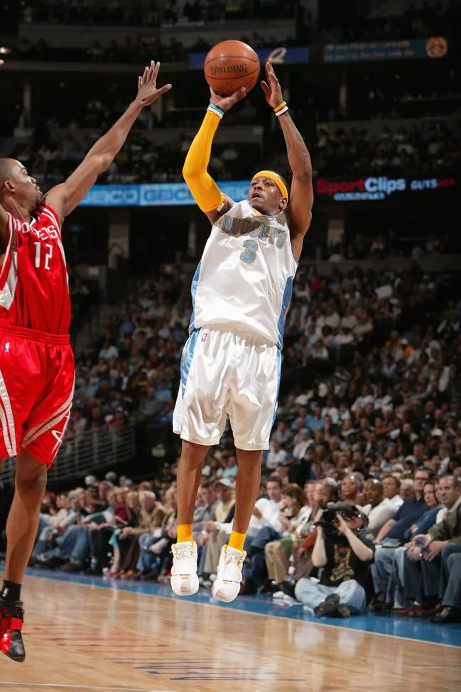
한 시대를 풍미했던, NBA 선수 엘런 아이버슨의 말이다. 하지만 3미터 위에 있는 골대에 슛을 넣기 위해서는, 나는 조금 다른 말을 하고 싶다.

'농구는 신장과 심장으로 한다.'

'아 물론, 엘런 아이버슨은 심장만으로 하셔도 됩니다.'

왜냐하면 결국 키가 크면 슛을 성공시킬 확률이 높기 때문이며, 엘런 아이버슨이 저런 말을 할 수 있는 것도 그가 굉장히 슛을 많이 성공시켰기 때문이다.

그렇기에,

농구에서 가장 중요한 것은 슛이다.

모든 볼 게임이 마찬가지 이듯, 슛을 성공해서 득점을 상대팀보다 조금이라도 더 많이 쌓아야 이긴다. 하지만 우리가 가장 많이 알고 있는 축구와 핸드볼과 비교할 때 가장 큰 차이점은, 농구의 골대는 터무늬 없이 작다는 것이다. 축구 골대의 높이가 2.44m, 폭은 7.32m, 핸드볼 골대는 가로 3m, 세로 2m인데 반해, 농구 골대의 림은 지름이 고작 **45cm**이다. 물론 농구 공의 지름이 27cm밖에 되지 않지만, 그럼에도 불구하고 다른 스포츠와 비교하면 굉장히 작은 것이 사실이다.
따라서 **슛의 성공률을 어떻게 하면 높일 수 있는 지**는 모든 농구하는 사람들의 공통적인 관심사라고 할 수 있다.
그리고 농구하면 '전세계에서 농구를 가장 잘하는 사람들이 모인 리그'라고 할 수 있는 NBA를 빼 놓을 수 없다. 그렇기에, 이번에 사용할 데이터는 NBA 데이터이다.

# DATA collection

```py
from google.colab import files
files.upload()
!mkdir -p ~/.kaggle
!cp kaggle.json ~/.kaggle/
!chmod 600 ~/.kaggle/kaggle.json
!kaggle datasets download -d dansbecker/nba-shot-logs
!kaggle datasets download -d justinas/nba-players-data
!unzip nba-players-data.zip
!unzip nba-shot-logs.zip
!pip install nba_api
```
우선 kaggle에서 데이터를 가져오려면 file upload를 통해서 kaggle.json을 넣으면 kaggle 데이터를 쉽게 업로드 할 수 있다.

그리고 사용하려던 주 데이터 shot log에는 선수들의 신체정보가 없기 때문에 선수들의 신체 정보를 얻기 위해 kaggle에 있는 NBA Players 데이터를 추가로 사용했다. 하지만 NBA Players data에는 player_id가 없기 때문에 shot log와 NBA player data를 매칭 시키기 위해서 nba_api에서 id와 이름 정보를 추가로 사용해야 했다.
```py
from nba_api.stats.static import players
import numpy as np
import pandas as pd
pd.options.mode.chained_assignment = None # default='warn'
df=pd.read_csv("shot_logs.csv")
df.columns=df.columns.str.lower()# 이름들을 소문자로 바꿔줍니다.
df.drop(columns=['player_name','closest_defender'],inplace=True)# 이름을 다시 붙이기 위해 없애줍니다.
df.drop(columns=['pts','shot_result'],inplace=True) # target을 100% 예측할 수 있기 때문에 제외했습니다.
df.drop(columns=['location','w'],inplace=True) # target을 100% 예측할 수 있기 때문에 제외했습니다.
df=df[df['touch_time']>0] # tocuh time이 음수인 것들을 제거. 기록상의 미스인지는 모르겠으나, 306개 밖에 안되서 데이터에 지장이 없을 것이다.

df_all=pd.read_csv("all_seasons.csv")
df_all=df_all[df_all['season']=='2014-15'] # shot_log data가 2014-2015년도까지만 있기 때문에 그때 활동한 선수들만 기록합니다.
df_all=df_all[['player_name','player_height','player_weight']]# 선수들의 이름, 키,몸무게만 남겨둡니다.

player_dict= pd.DataFrame(players.get_players())# get_players 에서 선수들의 id, 이름 정보를 가져옵니다.
player_dict.drop(columns=['first_name','last_name','is_active'],inplace=True)#이름와 id만 가져옵니다.
player_dict.columns=['id','player_name']#나중에 marge를 위해 이름을 바꿔줍니다.

list_id=list(set(df['closest_defender_player_id']) | set(df['player_id'])) # shot_log 에 있는 id들을 간추립니다.

player_dict=player_dict[player_dict['id'].isin(list_id)]# 먼저 id가 존재하는 log만 남깁니다.

player_dict['player_name']=player_dict['player_name'].str.lower() #모든 이름을 lower case로 바꿔줍니다.
df_all['player_name']=df_all['player_name'].str.lower()

exist_player=list(df_all['player_name'].unique())
player_dict=player_dict[player_dict['player_name'].isin(exist_player)]# all_seaons 에 있는 선수들만 간추립니다.
player_info=pd.merge(df_all,player_dict,on='player_name')
player_info.columns=['player_name', 'player_height', 'player_weight', 'player_id']
d_player_info=player_info.copy()
d_player_info.columns=['closest_defender_player_name', 'closest_defender_player_height', 'closest_defender_player_weight', 'closest_defender_player_id']

list_ex=list(player_info['player_id'])
df=df[df['closest_defender_player_id'].isin(list_ex)]
df=df[df['player_id'].isin(list_ex)]

# df.drop(columns=['game_id','matchup'],axis=1,inplace=True)
df.drop(columns=['matchup'],axis=1,inplace=True)
target='fgm' # target 은 fgm = field goal made 이다.
df=pd.merge(player_info.drop(columns='player_name'),df,on='player_id')
df=pd.merge(d_player_info.drop(columns='closest_defender_player_name'),df,on='closest_defender_player_id')
```
  | closest_defender_player_height | closest_defender_player_weight | closest_defender_player_id | player_height | player_weight | player_id | game_id | final_margin | shot_number | period | game_clock | shot_clock | dribbles | touch_time | shot_dist | pts_type | close_def_dist | fgm
-- | -- | -- | -- | -- | -- | -- | -- | -- | -- | -- | -- | -- | -- | -- | -- | -- | -- | --
190.50 | 90.71840 | 101114 | 190.50 | 86.18248 | 201565 | 21400467 | -14 | 4 | 2 | 8:14 | 4.5 | 0 | 1.1 | 23.9 | 3 | 9.7 | 0
190.50 | 90.71840 | 101114 | 190.50 | 86.18248 | 201565 | 21400467 | -14 | 5 | 2 | 7:03 | 13.0 | 12 | 11.6 | 10.9 | 2 | 1.3 | 0
190.50 | 90.71840 | 101114 | 190.50 | 86.18248 | 201565 | 21400467 | -14 | 6 | 2 | 5:04 | 20.1 | 4 | 2.4 | 18.2 | 2 | 4.6 | 0
190.50 | 90.71840 | 101114 | 190.50 | 86.18248 | 201565 | 21400320 | 25 | 1 | 1 | 11:07 | 6.7 | 0 | 1.2 | 25.0 | 3 | 1.8 | 0
190.50 | 90.71840 | 101114 | 190.50 | 86.18248 | 201565 | 21400320 | 25 | 2 | 1 | 5:21 | 17.0 | 7 | 7.4 | 5.6 | 2 | 0.7 | 1
... | ... | ... | ... | ... | ... | ... | ... | ... | ... | ... | ... | ... | ... | ... | ... | ... | ...
193.04 | 88.45044 | 202322 | 187.96 | 79.37860 | 202708 | 21400250 | -21 | 3 | 2 | 3:58 | 15.6 | 7 | 5.3 | 15.7 | 2 | 4.0 | 0
193.04 | 88.45044 | 202322 | 187.96 | 79.37860 | 202708 | 21400007 | 12 | 3 | 1 | 5:17 | 22.3 | 3 | 3.7 | 1.4 | 2 | 2.1 | 1
193.04 | 88.45044 | 202322 | 187.96 | 79.37860 | 202708 | 21400007 | 12 | 4 | 1 | 4:42 | 4.8 | 0 | 0.7 | 25.6 | 3 | 5.3 | 1
193.04 | 88.45044 | 202322 | 187.96 | 79.37860 | 202708 | 21400007 | 12 | 11 | 3 | 8:01 | 5.0 | 1 | 1.4 | 20.7 | 2 | 10.6 | 1
193.04 | 88.45044 | 202322 | 195.58 | 95.25432 | 201564 | 21400190 | -11 | 6 | 3 | 2:22 | 13.0 | 11 | 10.8 | 9.8 | 2 | 2.1 | 1

## DATA description

closest_defender_player_height: 가장 가까운 거리에 있는 수비수의 키. (단위:cm)
closest_defender_player_weight: 가장 가까운 거리에 있는 수비수의 몸무게. (단위:kg)
closest_defender_player_id: 가장 가까운 거리에 있는 수비수의 id
player_height: 슛을 시도하는 선수의 키.(단위:cm)
player_weight:슛을 시도하는 선수의 몸무게.(단위:kg)
game_id: NBA에서 부여한 게임의 id
final_margin:슛을 시도하는 선수가 경기가 끝났을 때, 그 선수가 플레이하고 있었을 때 상대팀과의 점수차가 얼마나 차이가 났는지를 표기(ex.) 선수가 뛰고 있을 동안 팀의 득점:28점, 상대팀의 득점: 34점, final_margin: -6점 )
shot_number: 슛을 시도하는 선수가 그 경기에서 몇번 째로 시도하는 슛인지
period: 총 4개의 정규 period, 이후 연장 period가 존재. 순서대로 1,2,3,4이며, 각 쿼터당 12분씩이다.
game_clock: 그 period에 남아있는 시간
dribble: 슛을 하기 전까지 몇번의 드리블을 했는지, 공을 바닥에 튀긴 횟수
touch_time: 슛을 하기 전까지 공을 소유하는 시간(단위: sec)
shot_dist: 슛을 시도할 때 선수와 림 사이의 거리(단위:M)
pts_type: 슛을 3점 라인 밖에서 했는지, 안에서 했는지.
close_def_dist:슛을 시도한 선수와 가장 가까운 수비자의 거리(단위:M)
fgm: field goal made. 슛을 성공 시켰는지의 여부(0: 실패, 1: t성공)

## DATA engineering

```py
def engineer(dfe):
dfe['closest_defender_player_height']=dfe['closest_defender_player_height'].copy()*0.0328084 # 키를 m단위로 변경
dfe['player_height']=dfe['player_height']*0.01
dfe['player_height_diff']=dfe['player_height']-dfe['closest_defender_player_height']
gtime=pd.DataFrame()
df['game_clock']=df['game_clock'].fillna(0)
df['shot_clock']=df['shot_clock'].fillna(0)
gtime[['m','s']]=df['game_clock'].str.split(':',n=2,expand=True)
dfe['g_clock']=gtime['m'].astype(int)*60+gtime['s'].astype(int)
dfe.drop(columns='game_clock',inplace=True)
dfe['shot_quality']=3 # average condtion
dfe['shot_quality'][dfe['close_def_dist']<=3.5]=2 #contest가 있음
dfe['shot_quality'][dfe['close_def_dist']<=2]=1 #contest가 심함
dfe['shot_quality'][dfe['close_def_dist']>6]=4 # wide open

return dfe
df=engineer(df)
```
1. 가장 먼저 한 것은 선수들의 키 단위를 cm->m로 바꿔주었다.
2. game_clock은 @@:@@, object로 되어있기 때문에, sec로 통일해 준다.
3. shot_quality는 슛을 시도하는 선수와 수비수의 거리가 얼마나 먼 지에 따라서 정했다.

## EDA

```py
import seaborn as sns
import matplotlib.pyplot as plt
import warnings
warnings.simplefilter(action='ignore', category=FutureWarning)
def eda_fgm(feat):
plt.figure(figsize=(10,10))
sns.distplot(df[feat][df['fgm']==1],label='sucess')
sns.distplot(df[feat][df['fgm']==0],label='fail')
plt.legend()
```

### player_height_diff

```py
feat='player_height_diff'
eda_fgm(feat)
```


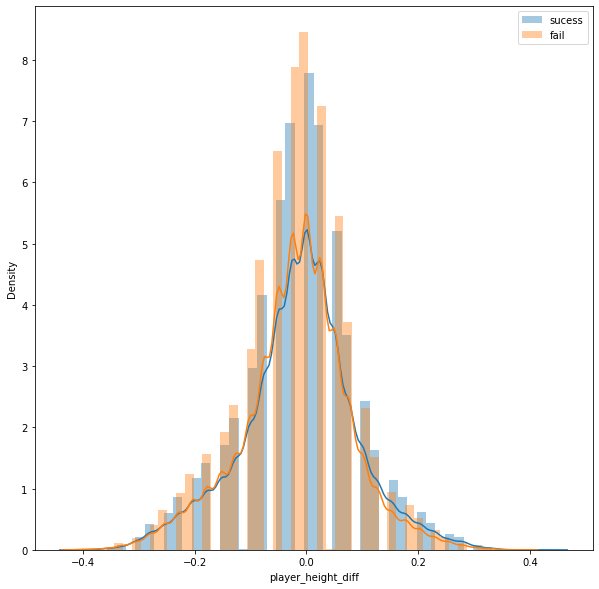
키 차이에 의한 성공확률이 크게 차이날 줄 알았지만, 의외로 정규분포를 따라가는 모양새였다. 다만, 슛하는 선수가 수비자보다 크면 조금씩 더 성공하는 모습을 보여주기는 한다. 마찬가지로, 수비하는 선수가 슛하는 선수보다 크면 슛이 실패하는 횟수가 늘긴 하지만 결정적인 요인은 아닌 것 처럼 보인다.

### final_margin

```py
feat='final_margin'
eda_fgm(feat)
plt.xlim(-30,30)
```


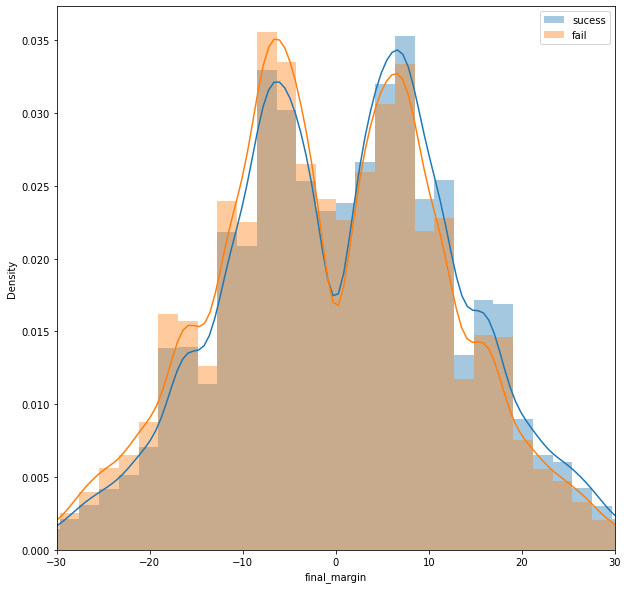
선수가 경기에서 뛰고 있을 때 팀이 얼마나 더 많은 점수를 획득했는지 역시 슛 성공률에서는 약간의 차이만 있었다. final_margin이 양수이면 슛을 성공할 확률이 조금 높았고, final_margin이 음수이면 슛을 실패할 확율이 조금 높았다.

### shot_clock

```py
feat='shot_clock'
eda_fgm(feat)
```

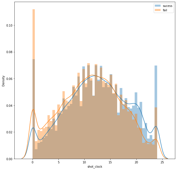
어찌보면 당연할 수도 있겠지만, 농구는 대부분의 공격이 10초 이내로 이루어진다. 그 이유는 준비된 패턴(선수들의 순서에 따라 정해지는 움직임)을 수행하는데 있어서 7~8초이면 충분하기 때문이다. 그게 실제로 성공횟수가 더 많다. 반대로 13초 안 쪽으로 공격 시간이 진행된다는 것은 패턴이 실패해도 재정비 하는 시간이 없어서 공격자 개인의 역량에 기대야 하는 경우가 많고, 급하게 던져야 하는 경우가 많기 때문에, shot_clock=0에서 실패 확률이 가장 높은 것으로 보인다.

### EDA에 대한 평가

NBA 선수들은 마치 던져야 하니까 던진다라는 느낌을 많이 주었다. 높은 확률을 쫒기 보다는, 슛을 던져야하는 순간에는 상황을 신경쓰지 않고 무조건 시도한다는 느낌이다.

# Modeling

어떤 모델이 어울리는지 잘 알지 못하기 때문에,

## baseline model

```py

from sklearn.metrics import accuracy_score
#최빈값
baseline = df[target].mode()[0]
#예측값
y_pred = [baseline] * len(train[target])
print('baseline:',baseline)
print('baseline model accuracy :', round(accuracy_score(train[target], y_pred)* 100,2),'%')

```
```py
baseline: 0
baseline model accuracy : 55.06 %
```

## RandomforestClassifier


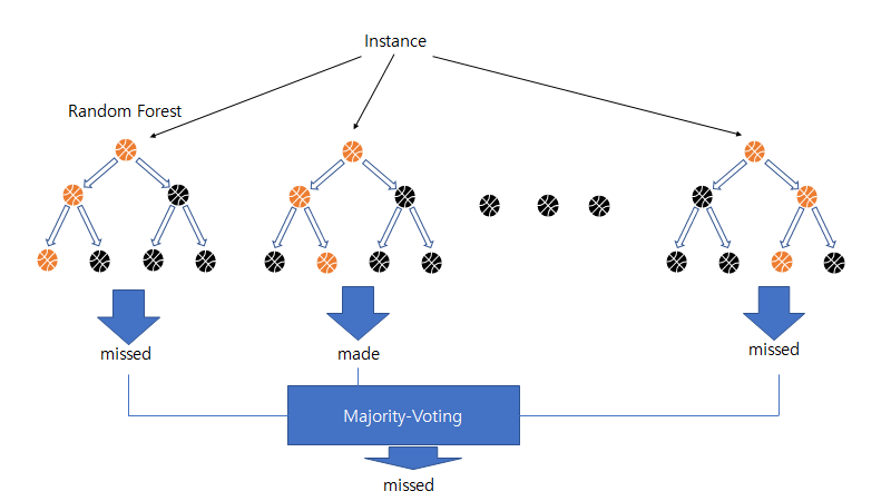
RandomforestClassifier은 여러개의 결정트리들을 무작위로 생성한 뒤, 각각의 트리에서 나온 결과들을 통해 Majority가 높은 class에 최종적으로 속하게 된다.

```py
import warnings
warnings.simplefilter(action='ignore', category=FutureWarning)
from category_encoders import HelmertEncoder
from sklearn.pipeline import make_pipeline
from sklearn.ensemble import RandomForestClassifier
from sklearn.metrics import accuracy_score, recall_score, precision_score, f1_score
from sklearn.impute import SimpleImputer

he_list=['closest_defender_player_id','player_id']
pipe=make_pipeline(
HelmertEncoder(),
SimpleImputer(),
RandomForestClassifier(n_jobs=-1,n_estimators=100,random_state=10)
)

pipe.fit(X_train,y_train)
print('검증 정확도: ', pipe.score(X_val, y_val))
y_pred=pipe.predict(X_train)
print('f1 train f1_score: ',f1_score(y_train, y_pred))
y_pred=pipe.predict(X_val)
from sklearn.metrics import classification_report
print(classification_report(y_val, y_pred))
```

```py
검증 정확도: 0.6113814074717637
f1 train f1_score: 1.0
precision recall f1-score support

0 0.61 0.79 0.69 12630
1 0.61 0.39 0.48 10390

accuracy 0.61 23020
macro avg 0.61 0.59 0.58 23020
weighted avg 0.61 0.61 0.59 23020
```

아무런 과적합 제어를 하지 않으니 overfitting이 되었고, train의 f1_score은 1이 되어버렸다. 그리고 validation set에 대한 f1_score은 0.475로 그렇게 좋은 성능이 아니라고 할 수 있다. 무엇보다, 과적합이 시각하기 때문에 ,과적합을 적절하게 제어하는 방향으로 모델을 다시 만들어 보았다.

```py
import warnings
warnings.simplefilter(action='ignore', category=FutureWarning)
from category_encoders import HelmertEncoder
from sklearn.pipeline import make_pipeline
from sklearn.ensemble import RandomForestClassifier
from sklearn.metrics import accuracy_score, recall_score, precision_score, f1_score
from sklearn.impute import SimpleImputer

he_list=['closest_defender_player_id','player_id']
pipe=make_pipeline(
HelmertEncoder(),
SimpleImputer(),
RandomForestClassifier(n_jobs=-1,n_estimators=400,min_samples_split=4,min_samples_leaf=4,max_depth=15,random_state=10)
)

pipe.fit(X_train,y_train)
print('검증 정확도: ', pipe.score(X_val, y_val))
y_pred=pipe.predict(X_train)
print('f1 train f1_score: ',f1_score(y_train, y_pred))
y_pred=pipe.predict(X_val)
print(classification_report(y_val, y_pred))
```
```py
검증 정확도: 0.6221112076455256
f1 train f1_score: 0.6512535045304945
precision recall f1-score support

0 0.61 0.85 0.71 12630
1 0.65 0.35 0.46 10390

accuracy 0.62 23020
macro avg 0.63 0.60 0.58 23020
weighted avg 0.63 0.62 0.60 23020

```
검증 정확도는 올라갔고, 과적합도 해결된 것 처럼 보이지만, validtaion set에서 그렇게 성능이 좋지 않았다.

두번째 모델을 통해 과적합을 줄이니 슛이 실패하는 것을 조금 더 잘 찾게 되었는데, 내가 원하는 것은 label의 값이 1 일 때 recall의 값을 높이는 것을 원하기 때문에, 오히려 overfiting하는 것이 나아보인다.

#### Test

```py
pipe=make_pipeline(
HelmertEncoder(),
SimpleImputer(),
RandomForestClassifier(n_jobs=-1,n_estimators=100,random_state=10)
)
pipe.fit(X_train,y_train)
y_pred=pipe.predict(X_test)
from sklearn.metrics import classification_report
print(classification_report(y_test, y_pred))
```
```py
precision recall f1-score support

0 0.61 0.80 0.69 16762
1 0.61 0.38 0.47 13932

accuracy 0.61 30694
macro avg 0.61 0.59 0.58 30694
weighted avg 0.61 0.61 0.59 30694

```
```py
```py
pipe=make_pipeline(
HelmertEncoder(),
SimpleImputer(),
RandomForestClassifier(n_jobs=-1,n_estimators=400,min_samples_split=4,min_samples_leaf=4,max_depth=15,random_state=10)
)
pipe.fit(X_train,y_train)
y_pred=pipe.predict(X_test)
from sklearn.metrics import classification_report
print(classification_report(y_test, y_pred))
```
```py
precision recall f1-score support

0 0.61 0.85 0.71 16762
1 0.66 0.35 0.45 13932

accuracy 0.62 30694
macro avg 0.63 0.60 0.58 30694
weighted avg 0.63 0.62 0.59 30694

```
실제로, Test를 돌려보니 overfitting이 된 모델의 1에대한 recall 값은 0.38, 파라미터를 조절한 모델의 1에 대한 recall 값은 0.35로 overfitting된 모델이 조금 더 좋아보인다.

## XGBoost


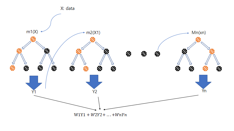
Boosting은 원리가 다른데 먼저 M1~n 모델이 있을때, M1에는 x에서 샘플링된 데이터를 넣는다. 그리고, 나온 결과중에서, 예측이 잘못된 x중의 값들에 가중치를 반영해서 다음 모델인 M2에 넣는다. 마찬가지로 y2 결과에서 예측이 잘못된 x’의 값들에 가중치를 반영해서 m-3에 넣는다. 그리고 이 것을 반복해서 Mn까지 가게되고, 그 때 선택된 값이 최종 선택 값이 된다.
그리고, 각 모델의 성능이 다르기 때문에, 각 모델에 가중치 W를 반영한다.

```py
import xgboost as xgb

pipe_x=make_pipeline(
HelmertEncoder(),
SimpleImputer(),
xgb.XGBClassifier(n_jobs=-1,booster='gbtree',random_state=10)
)
pipe_x.fit(X_train,y_train)
print('검증 정확도: ', pipe_x.score(X_val, y_val))
y_pred=pipe_x.predict(X_train)
print('f1 train f1_score: ',f1_score(y_train, y_pred))
y_pred=pipe_x.predict(X_val)
from sklearn.metrics import classification_report
print(classification_report(y_val, y_pred))
```
```py
검증 정확도: 0.6248479582971329
f1 train f1_score: 0.45791717030345436
precision recall f1-score support

0 0.61 0.86 0.71 12630
1 0.66 0.34 0.45 10390

accuracy 0.62 23020
macro avg 0.64 0.60 0.58 23020
weighted avg 0.64 0.62 0.60 23020
```

```py
import xgboost as xgb

pipe_x=make_pipeline(
HelmertEncoder(),
SimpleImputer(),
xgb.XGBClassifier(n_jobs=-1,booster='gbtree',n_estimators=400,min_child_weight=6,max_depth=5,colsample_bytree=0.8,colsample_bylevel=0.9,silent=True,gamma=1,random_state=10)
)
pipe_x.fit(X_train,y_train)
print('검증 정확도: ', pipe_x.score(X_val, y_val))
y_pred=pipe_x.predict(X_train)
print('f1 train f1_score: ',f1_score(y_train, y_pred))
y_pred=pipe_x.predict(X_val)
print('f1 val f1_score: ',f1_score(y_val, y_pred))
```
```py
검증 정확도: 0.6171589921807125
f1 train f1_score: 0.5671641791044776
precision recall f1-score support

0 0.61 0.81 0.70 12630
1 0.62 0.38 0.47 10390

accuracy 0.62 23020
macro avg 0.62 0.60 0.59 23020
weighted avg 0.62 0.62 0.60 23020
```

파라미터를 조정했는데도, 성공에 대한 recall 이 0.38밖에 안된다. 잠깐 feature들을 살펴보자.
```py
### 이곳에서 과제를 진행해 주세요 ###
from category_encoders import OrdinalEncoder
from sklearn.metrics import r2_score

encoder = HelmertEncoder()
X_train_encoded = encoder.fit_transform(X_train) # 학습데이터
X_val_encoded = encoder.transform(X_val) # 검증데이터

# 기준 모델
boosting = xgb.XGBClassifier(n_jobs=-1,booster='gbtree',n_estimators=1000,min_child_weight=7,max_depth=5,colsample_bytree=0.5,colsample_bylevel=0.6,silent=True,gamma=0,random_state=2)
eval_set = [(X_train_encoded, y_train),
(X_val_encoded, y_val)]

# 모델 학습
boosting.fit(X_train_encoded, y_train,
eval_set=eval_set,
early_stopping_rounds=50
)
```
pdp isolate를 위한 함수를 만들어준다.
```py
from pdpbox.pdp import pdp_isolate, pdp_plot
import matplotlib.font_manager
def isol_pdp(feature):
isolated = pdp_isolate(
model=boosting,
dataset=X_val,
model_features=X_val.columns,
feature=feature)
pdp_plot(isolated, feature_name=feature);
```

``py
feature='player_height_diff'
isol_pdp(feature)
```

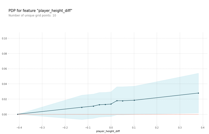
수비수보다 키가 클 수록 성공률이 높아진다.

```py
feature='close_def_dist'
isol_pdp(feature)
```

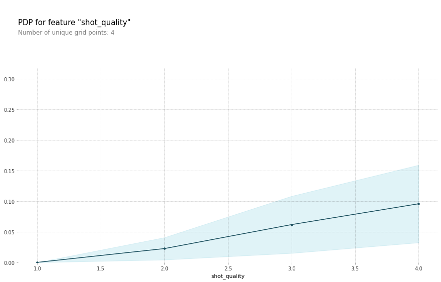
```py
feature='shot_quality'
isol_pdp(feature)
```

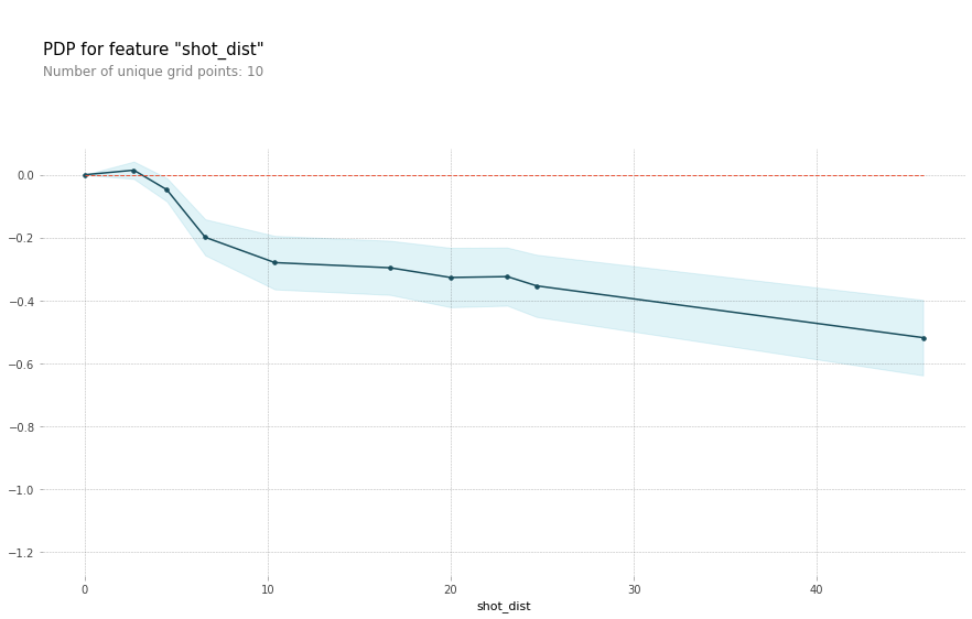
```py
feature='shot_dist'
isol_pdp(feature)
```

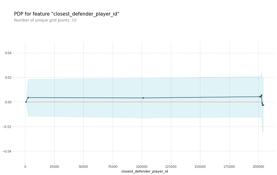
```py
feature='closest_defender_player_id'
isol_pdp(feature)
```

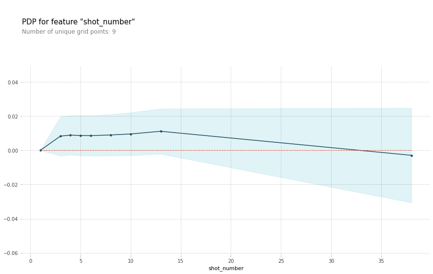
```py
feature='shot_number'
isol_pdp(feature)
```

## Permutation Importance

중요한 특성들이 있는 반면, 그렇지 못한 특성들도 분명히 존재한다. 물론 pdp를 사용해 하나하나 살펴보는 것도 좋겠지만, Permutation Importance를 사용해서 어떤 특성이 도움이 되는지, 어떤 특성이 도움이 안되는지를 바로 알아볼 수 있기 때문에 한 번 확인해보려고 한다.

```py
from sklearn.pipeline import Pipeline
pipe = Pipeline([
('preprocessing', make_pipeline(HelmertEncoder(), SimpleImputer())),
('xgb',xgb.XGBClassifier(n_jobs=-1,booster='gbtree',n_estimators=600,min_child_weight=7,max_depth=5,colsample_bytree=0.5,colsample_bylevel=0.6,silent=True,gamma=0,random_state=2))
], verbose=1)

pipe.fit(X_train, y_train);
```
준비는 간단하다. 데이터를 어떻게 가공할지와, 모델을 집어넣으면 된다.
```py
import warnings
warnings.simplefilter(action='ignore', category=FutureWarning)

import eli5
from eli5.sklearn import PermutationImportance

# permuter 정의
permuter = PermutationImportance(
pipe.named_steps['xgb'], # model
scoring='accuracy', # metric
n_iter=5, # 다른 random seed를 사용하여 5번 반복
random_state=2
)

X_val_transformed = pipe.named_steps['preprocessing'].transform(X_val)
# 우리가 아는 일반적인 fit이 아니고 스코어를 다시 계산하는 작업이다
permuter.fit(X_val_transformed, y_val);
feature_names = X_val.columns.tolist()
pd.Series(permuter.feature_importances_, feature_names).sort_values()
```
```py
closest_defender_player_id -0.001868
shot_number -0.001460
player_height_diff -0.001312
player_weight -0.001086
period -0.000773
game_id -0.000617
g_clock -0.000599
closest_defender_player_height -0.000443
player_id -0.000295
player_height 0.000582
shot_clock 0.000704
closest_defender_player_weight 0.000921
pts_type 0.001095
dribbles 0.001416
final_margin 0.001720
shot_quality 0.004179
close_def_dist 0.008471
touch_time 0.009687
shot_dist 0.085665
```

여기서 도움이 안되는, 음수로 값이 표시된 특성들을 제거하고 나머지로 다시 한번 모델을 돌려보았다.

```py
list_d=['player_height','shot_clock','closest_defender_player_weight','pts_type','player_height_diff','final_margin','touch_time','shot_quality','close_def_dist','shot_dist','dribbles']
from sklearn.model_selection import train_test_split

train,test=train_test_split(df)
train,val=train_test_split(train)

features=list_d
X_train=train[features]
y_train=train[target]
X_test=test[features]
y_test=test[target]
X_val=val[features]
y_val=val[target]
````
```py
import xgboost as xgb
pipe_x=make_pipeline(
HelmertEncoder(),
SimpleImputer(),
xgb.XGBClassifier(n_jobs=-1,booster='gbtree',n_estimators=1000,min_child_weight=7,max_depth=5,colsample_bytree=0.5,colsample_bylevel=0.6,silent=True,gamma=0,random_state=2)
)
pipe_x.fit(X_train,y_train)
print('검증 정확도: ', pipe_x.score(X_val, y_val))
y_pred=pipe_x.predict(X_train)
print('f1 train 검증 정확도: ',f1_score(y_train, y_pred))
y_pred=pipe_x.predict(X_val)
print(classification_report(y_val, y_pred))
```
```py
검증 정확도: 0.6108166811468289
f1 train 검증 정확도: 0.5846824768924994
precision recall f1-score support

0 0.61 0.79 0.69 12705
1 0.60 0.39 0.47 10315

accuracy 0.61 23020
macro avg 0.61 0.59 0.58 23020
weighted avg 0.61 0.61 0.59 23020
```

아직도 recall이 만족스럽지 못하다.

## LogisticRegression

randomforest와 XGBoost의 성능이 너무나도 안좋다고 판단해서, 이번에는 한번 Logistic Regression을 써보기로 했다.


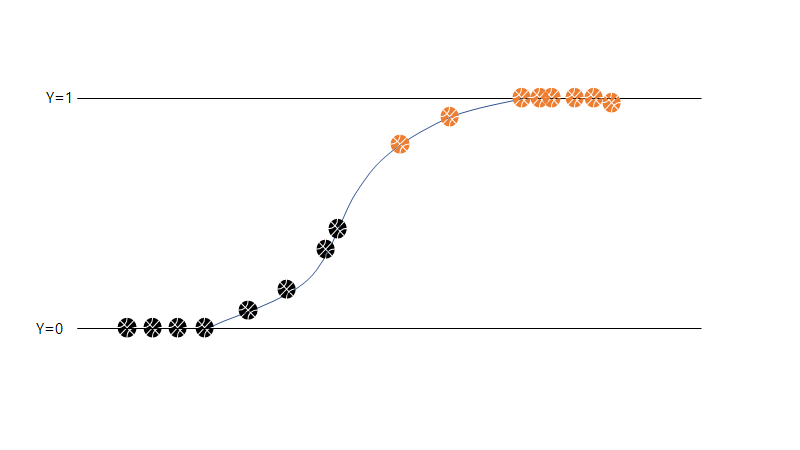
로지스틱 회귀(Logistic Regression)는 회귀를 사용하여 데이터가 어떤 범주에 속할 확률을 0에서 1 사이의 값으로 예측하고 그 확률에 따라 가능성이 더 높은 범주에 속하는 것으로 분류해주는 지도학습의 한 방법이다.

```py
from sklearn.preprocessing import StandardScaler
from sklearn.linear_model import LogisticRegression
pipe_l=make_pipeline(
HelmertEncoder(),
SimpleImputer(),
StandardScaler(),
LogisticRegression(random_state=0)
)
pipe_l.fit(X_train,y_train)
print('검증 정확도: ', pipe_x.score(X_val, y_val))
y_pred=pipe_l.predict(X_train)
print('f1 train 검증 정확도: ',f1_score(y_train, y_pred))
y_pred=pipe_l.predict(X_val)
print(classification_report(y_val, y_pred))
```
```py
검증 정확도: 0.6171589921807125
f1 train 검증 정확도: 0.5121270027928855
precision recall f1-score support

0 0.62 0.75 0.68 12630
1 0.59 0.45 0.51 10390

accuracy 0.61 23020
macro avg 0.61 0.60 0.59 23020
weighted avg 0.61 0.61 0.60 23020
```

RandomForest와 XGBoost보다 성능이 훨씬 더 좋아진 것을 관찰할 수 있었다. 한번 coefficent를 살펴보자.

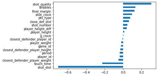
아까 Permutation Importance에서 중요하다고 판단한 특성들이 여기서도 높은 coefficient를 가진다. 아까처럼 특성들을 제한하고 다시 한번 모델을 돌려본 결과이다.
```py
검증 정확도: 0.6125977410947002
f1 train 검증 정확도: 0.5120765885920999
precision recall f1-score support

0 0.62 0.74 0.68 12558
1 0.60 0.46 0.52 10462

accuracy 0.61 23020
macro avg 0.61 0.60 0.60 23020
weighted avg 0.61 0.61 0.60 23020
```
아주 미세하게 좋아졌다. 다시 한번 coefficent를 확인해 보자.
```py
model=pipe_l.named_steps['logisticregression']
coefficients = pd.Series(model.coef_[0], X_train.columns)
coefficients.sort_values().plot.barh();
```

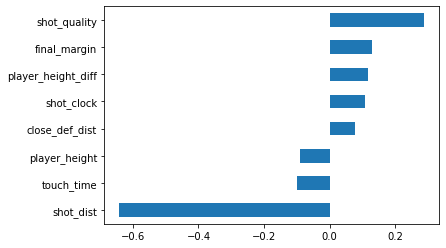
가장 결정적인 요인은 shot quality로, 컨테스트를 받지 않을수록 슛 성공률이 높아졌고, 반대로 shot_dist, 즉 슛을 쏘는 거리가 멀어질 수록 슛 성공률은 낮아졌다. 그리고 키차이도 어느정도 영향을 미쳤는데, NBA 선수들의 평균키가 2m 인 것을 감안하면 다들 너무 크기 때문에 오히려 영향을 적게 받는 것 같다.

## 최종 모델 테스트

```py
y_pred=pipe_l.predict(X_test)
print(classification_report(y_test, y_pred))
```
```py
precision recall f1-score support

0 0.63 0.74 0.68 16937
1 0.59 0.45 0.51 13757

accuracy 0.61 30694
macro avg 0.61 0.60 0.59 30694
weighted avg 0.61 0.61 0.60 30694
```

# 결론

처음에는, 슛 성공에 대한 recall이 굉장히 낮게 나와서 굉장히 낙담을 했었다. 내가 feature들을 잘못 선택한건가? 모델이 적합하지 않았나? 며칠을 고민하다가, 드디어 깨달았다.
아닌 것은 확실하게 아니라고 말할 수 있다. 그러나 성공에 대해서는, 대상이 NBA 선수들이기 때문에, 모델이 전혀 슛을 성공 시킬 수 없다고 판단을 하는데도 기어코 성공하는 NBA 선수들이 있기 때문에 모델이 성공에 대한 예측을 잘 하지 못하는 것 같다.

즉, NBA 선수들은 **'불가능'을 '가능'으로 만드는** 사람들이고, 그렇기에 NBA는 꿈의 무대라는 말이 어울린다고 생각한다.

**"the shot" : 수비수가 앞에서 막고 있음에도 버져비터 슛을 성공시키는 마이클 조던**